
A meta-analysis, also written as meta analysis, is a statistical procedure that combines the results of two or more separate studies into one estimate. It is a calculation, normally run inside a systematic review, that decides which studies go into it.
The distinction matters because the calculation is the easy part. Chapter 10 of the Cochrane Handbook (the Handbook) opens with a section titled “Do not start here!”, and the warning holds. A pooled estimate is only as sound as the question, the search, the screening, and the extraction beneath it.
This guide moves from definition to practice: reading a forest plot, pooling, heterogeneity, the two models, and the data that is needed first.
What a meta-analysis is and what it is not
The opening definition is close to the Handbook’s wording, and it is narrow on purpose. A meta-analysis takes an effect estimate and its precision from each study, weights them, and returns an average with a confidence interval.
A systematic review is the larger method around it: the protocol, the search, dual screening, extraction, and appraisal. A meta-analysis run without one inherits every bias in how its studies were chosen.
The reverse does not hold. Many systematic reviews contain no meta-analysis, because their studies ask different questions or measure outcomes that cannot share a scale. Those reviews synthesize narratively, and that is a legitimate result.
Cochrane lists three potential gains: more precision than any single study, answers to questions no study posed, and a way to settle conflicting claims. The same chapter warns that a meta-analysis can also mislead, when study design, bias within studies, variation between them, and reporting bias are ignored.
The term began in education and psychology research. Gene Glass coined it in 1976 for the analysis of analyses: statistical work on the results of many individual studies, done to integrate their findings.
Examples of meta-analyses
In psychology, Smith and Glass published “Meta-analysis of psychotherapy outcome studies” in American Psychologist in 1977. It pooled controlled evaluations of psychotherapy and counseling, one of the method’s first applications.
In medicine, one example of a meta-analysis is printed on Cochrane’s logo. The logo is a stylized forest plot from a systematic review of corticosteroids given before a premature birth. As Cochrane recounts in its own history, the treatment saves infants’ lives.
A meta-analysis of meta-analyses
A meta-analysis of meta-analyses, sometimes called a meta-meta-analysis, pools or compares the results of existing reviews in place of primary studies. Cochrane calls the broader form an overview of reviews, and JBI calls it an umbrella review. The main hazard is overlap: one trial can appear in several source reviews and be counted more than once.
How to read a forest plot
A forest plot shows every study in a meta-analysis on one shared axis, with the pooled result underneath. The example below is illustrative: seven constructed studies, each reporting a risk ratio (RR). An RR is the risk of the outcome in the intervention group divided by the risk in the comparator group.
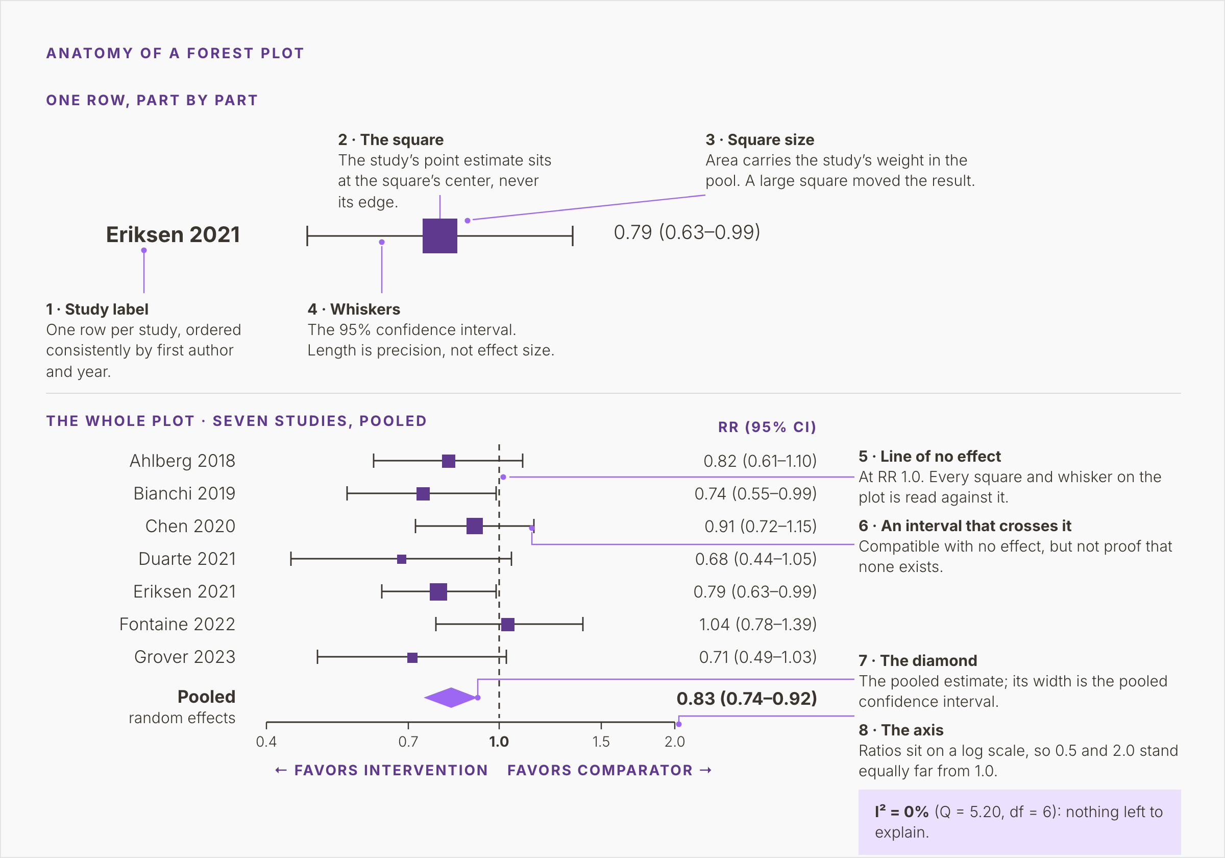
Figure 1. Seven illustrative studies and their pooled random-effects estimate, RR 0.83 (0.74–0.92), with eight numbered callouts naming each part of the plot and I² = 0%.
Study labels, squares, and weight
Each row is one study, labeled by first author and year, from Ahlberg 2018 down to Grover 2023. The order should be consistent, e.g., by year, by weight, or alphabetically, so a reader can scan it.
The square marks the study’s point estimate. Read its center and ignore its edges. Eriksen 2021 sits at a risk ratio of 0.79, and the printed column gives its interval as 0.63 to 0.99.
Square size carries weight. Precise studies count for more, and the area of each square is drawn in proportion to its weight.
Working back from the printed intervals, Eriksen 2021 and Chen 2020 carry about a fifth of the weight each. Duarte 2021 carries about six percent. A large square marks a study that moved the pooled result, and a small square marks one that barely moved it.
Whiskers and the line of no effect
The horizontal line through each square is its 95% confidence interval. Its length reflects precision: short whiskers mean a precise estimate, long whiskers an imprecise one. Length says nothing about how large the effect is.
The vertical line at 1.0 is the line of no effect. A risk ratio of 1.0 means the outcome was equally likely in both groups. In this plot, estimates left of the line favor the intervention and those to the right favor the comparator. For difference measures, such as a mean difference, the line sits at zero.
Five of the seven intervals cross the line: Ahlberg, Chen, Duarte, Fontaine, and Grover. Each is compatible with no effect, which is weaker than showing there is none. Duarte 2021 has a point estimate of 0.68. Its interval runs from 0.44 to 1.05, a 56 percent lower risk to a five percent higher one. On its own, the study cannot separate a large benefit from none. Pooling exists to deal with that imprecision.
The diamond
The diamond at the foot of the plot is the pooled estimate. Its center is the point estimate, and its width is the pooled confidence interval. Here it reads 0.83 (0.74 to 0.92), from a random-effects model.
Read that as a risk about 17 percent lower with the intervention, with an interval from eight to 26 percent lower. The diamond is narrower than any single study’s interval. It sits clear of the line of no effect, although five of the seven studies do not.
Pooling gains precision this way. It also carries every flaw of the pooled studies into the result. That is why risk of bias is assessed before the diamond is drawn.
The axis and the heterogeneity statistics
Ratios are plotted on a log scale. On that scale 0.5 and 2.0 sit equally far from 1.0. Halving a risk and doubling it are effects of equal size in opposite directions. That is why the gaps between the figure’s ticks are uneven.
Check the axis labels as well. The authors decide which side favors which arm, and some plots put benefit on the right.
Cochrane-style forest plots print heterogeneity statistics under the pooled result. This one gives I² = 0%, with Q = 5.20 on six degrees of freedom.
From studies to a pooled estimate
Five steps lead from the included studies to the diamond. The first belongs to the review team. The rest belong to the statistics package.
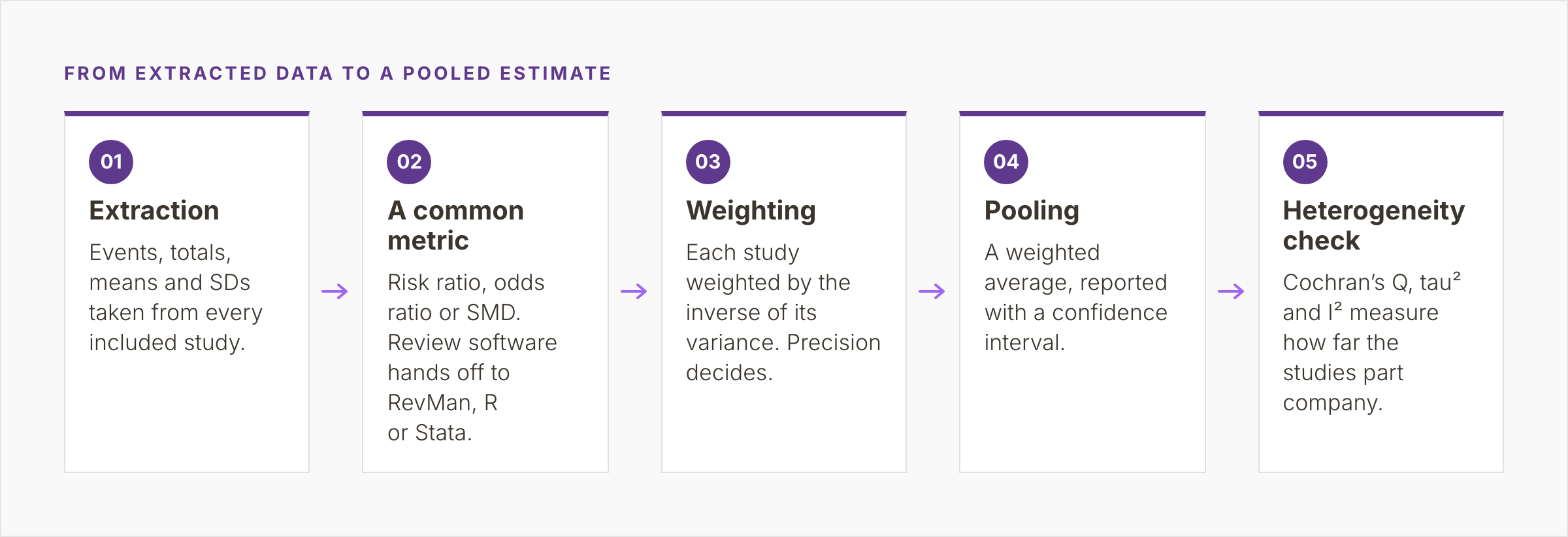
Figure 2. Five steps from extraction through a common metric, inverse-variance weighting and pooling to a heterogeneity check, with the handoff from review software to RevMan, R, or Stata at step two.
Extraction and a common metric
Extraction pulls the raw numbers from every included study. For a binary outcome, that means events and totals in each arm. For a continuous outcome, it means the mean, the standard deviation, and the number of participants in each arm. Studies that report only an effect estimate need its standard error or confidence interval as well.
Those numbers are then converted to one effect measure. Binary outcomes become a risk ratio or an odds ratio. Continuous outcomes become a mean difference or a standardized mean difference (SMD). The SMD divides each study’s difference in means by the standard deviation of the outcome among its participants. Studies that measure one construct on different scales can then be pooled. Ratio measures are analyzed as natural logarithms and reported back on the original scale.
Weighting and pooling
Each study gets a weight equal to one divided by the variance of its estimate, the square of its standard error. A large study with many events has a small variance and a large weight. This is the inverse-variance method, which runs behind many meta-analyses of binary and continuous data.
Pooling is then a weighted average of the study estimates, reported with its confidence interval. For binary outcomes with few events, the Mantel-Haenszel method has better statistical properties. The Handbook generally prefers it for fixed-effect analyses of binary data.
The last step checks, with Cochran’s Q, tau² and I², whether the studies agree well enough for one average to mean anything.
Heterogeneity: what I² tells you
Heterogeneity is variation between study results beyond what chance would produce. It comes from clinical differences in population, dose or follow-up, and from differences in design and risk of bias.
Q, tau², and I²
Cochran’s Q sums the weighted squared distances of each study from the fixed-effect pooled estimate. If every study shared one true effect, Q would be expected to equal its degrees of freedom, the number of studies minus one.
The test built on Q has low power when studies are few or small, so a non-significant result proves little.
Tau² estimates the variance of the true effects across studies, on the scale of the analysis. It drives the random-effects model in the next section.
Higgins and Thompson introduced I² in 2002. It takes Q minus its degrees of freedom, divides by Q, and sets the result to zero when Q falls below the degrees of freedom. It is the percentage of variability in effect estimates due to heterogeneity and not to chance.
In the forest plot above, Q (5.20) is below its six degrees of freedom, so I² is zero percent.
How to read I²
Higgins and colleagues, in a 2003 BMJ paper, tentatively labeled I² values of 25%, 50%, and 75% as low, moderate, and high. The Handbook’s rough guide uses overlapping bands: zero to 40% might not be important, and 30 to 60% may be moderate. From 50 to 90% heterogeneity may be substantial, and 75 to 100% is considerable. The Handbook warns that thresholds can mislead. The importance of I² depends on the size and direction of the effects, and on the strength of evidence for heterogeneity.
I² is itself uncertain when studies are few. A value of zero percent from seven studies is an estimate with a wide interval of its own. I² measures inconsistency as a proportion. Tau² and the prediction interval show how far apart the true effects lie.
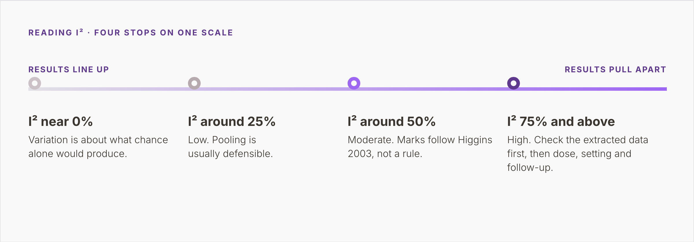
Figure 3. One scale with four stops, from I² near 0%, where variation matches chance, to 75% and above, where the extracted data are checked first, then dose, setting and follow-up length.
No rule fixes the point where pooling stops being defensible. The decision figure in the next section draws its working line at 75 percent, Higgins’s high mark and the start of Cochrane’s considerable band. Above it, the data are checked first, because severe apparent heterogeneity can signal extraction errors. Dose, setting, and follow-up length are then examined through subgroup analyses or meta-regression planned in the protocol. Sensitivity analyses test whether the result holds up.
Fixed effect or random effects
Most meta-analyses rest on one of two models. When tau² is above zero, the choice changes both the weights and the width of the diamond.
What each model assumes
A fixed-effect model assumes one true effect behind every study, so differences between results are chance alone. It suits studies of the same population, dose and outcome.
A random-effects model assumes the true effects vary and the studies sample a distribution of them. It adds tau² to every study’s variance, which gives small studies more weight and widens the interval once tau² rises above zero. Higgins and colleagues argue that clinical and methodological diversity make some heterogeneity inevitable.
The two models give identical results when there is no heterogeneity. The random-effects diamond in the forest plot above, with I² at zero percent, is therefore the fixed-effect diamond as well. The Handbook is firm that the choice between them should never rest on a statistical test for heterogeneity. It belongs in the protocol.
A random-effects estimate describes the center of the distribution of effects. Its spread needs the prediction interval, the range in which the true effect in a new, similar study would be expected to lie. The Handbook encourages it with five or more studies and no clear funnel plot asymmetry.
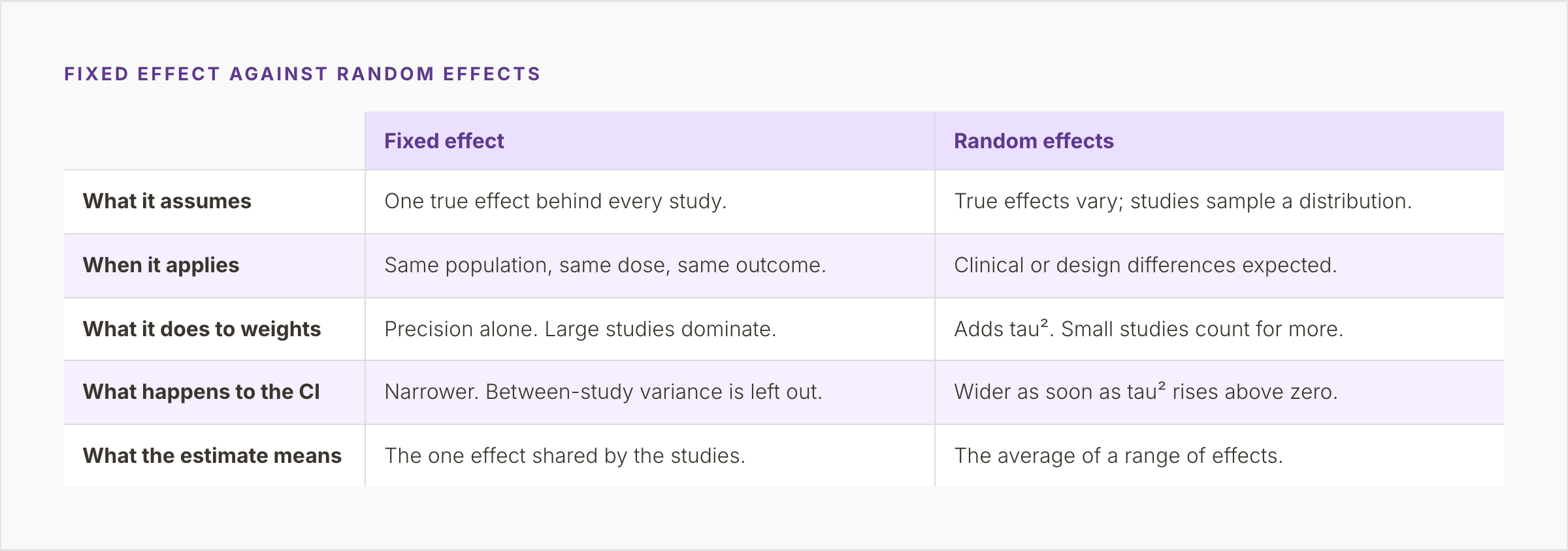
Figure 4. A two-column comparison of what each model assumes, when it applies, what it does to study weights and to the confidence interval, and what its estimate means.
When there are very few studies
A random-effects model needs an estimate of tau², and with few studies that estimate is poor. The Handbook says fixed-effect methods, such as Mantel-Haenszel, then give “more robust estimates of the average intervention effect”, but ignore heterogeneity. Borenstein and colleagues, in “Introduction to Meta-Analysis”, list the same option alongside two others: report the studies without a summary, or take a Bayesian approach.
The Handbook also describes the Hartung-Knapp-Sidik-Jonkman (HKSJ) adjustment, which generally widens the random-effects interval to reflect uncertainty in tau². It has limits at both ends. When tau² is estimated at zero, as in the example above, it can give an interval that is too narrow. With two or three studies it can give one that is excessively wide, and the Handbook advises a sensitivity analysis comparing methods. Whichever route the team takes, the protocol should name it before the data are seen.
The figure below puts the decision in one place: four questions, each with its exit.
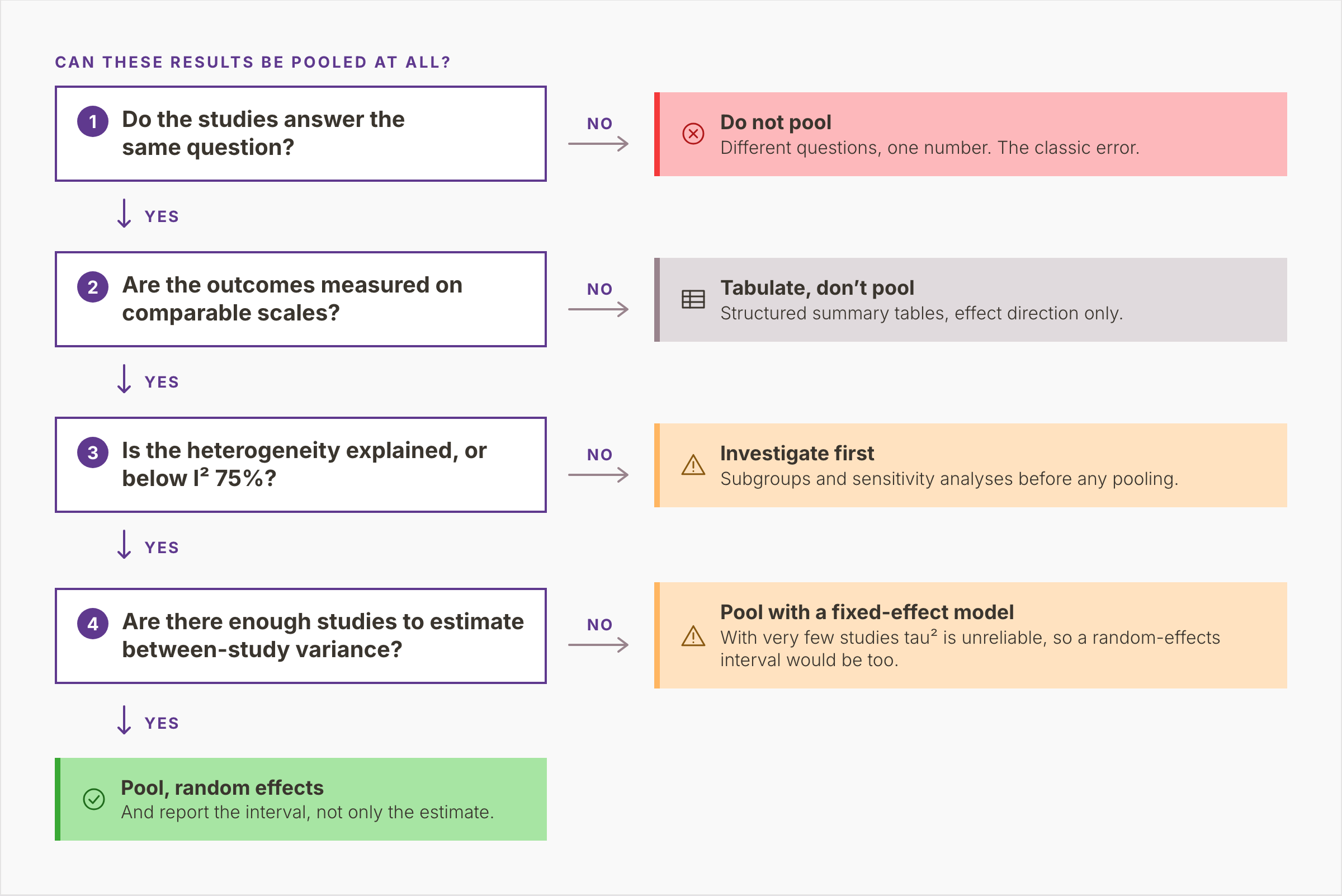
Figure 5. Four questions in sequence, on the question, the outcome scales, heterogeneity and the number of studies, each with its exit, ending in a random-effects pool reported with its interval.
Publication bias and the funnel plot
A meta-analysis can only pool what was reported. When small studies with null or unfavorable results stay unpublished, the pooled estimate tends to overstate the effect.
A funnel plot checks for this. It plots each study’s effect estimate on the horizontal axis against its standard error on the vertical. The vertical scale is reversed, so the largest studies sit at the top. Without bias, the points form a symmetric inverted funnel. Large studies cluster near the pooled effect and small ones scatter widely on both sides.
Asymmetry usually shows as a gap in one bottom corner, where small studies without significant results would have been. Chapter 13 of the Handbook reads asymmetry as a sign of small-study effects, which have several causes besides non-reporting. Small studies with unblinded outcome assessment can exaggerate effects, and true heterogeneity or chance can tilt the plot as well.
Formal tests exist, and Egger’s test is the best known. Following Sterne and colleagues, the Handbook advises using them only with at least 10 studies, and not when the studies are of similar size. Citing Nguyen and colleagues (2022), the chapter notes that only 28% of 300 randomly sampled systematic reviews indexed in 2020 had a meta-analysis that large. The seven-study example above falls below that line.
Extracted data you need before pooling
Every calculation above runs on extracted numbers, and no statistics package repairs inconsistent extraction. Four things need to be in place first:
One extraction form for every study. The same fields, units, and definitions, filled in by two reviewers independently, and then reconciled. Two reviewers working in their own spreadsheets produce two schemas.
The fields the analysis needs. Events and totals per arm for binary outcomes; means, standard deviations, and numbers per arm for continuous ones. Some studies omit the standard deviation. Chapter 6 of the Handbook shows how to derive it from a standard error, confidence interval, or P value.
Decisions recorded before the data are seen. Which time point, which outcome definition, which arm counts as the comparator, and which direction on a scale counts as better. Each choice changes the numbers that enter the plot.
A statistician involved before extraction. The fields needed for pooling define the form. Adding them later means returning to every included study.
The studies that reach extraction are the ones your PRISMA 2020 flow diagram reports as included. Each meta-analysis draws on some or all of them, and the report should say which. In PICO Portal, extraction runs on pre-built or custom forms, with dual independent review as an option. Both reviewers fill in the same fields for every study, and an adjudicator resolves discrepancies. The documentation shows how extraction forms are configured.
Software for pooling: RevMan, R, and Stata
Three statistics packages are in wide use:
RevMan. Cochrane’s Review Manager, used to prepare Cochrane reviews, draws forest and funnel plots in the Cochrane format. Since 2024, it estimates tau² by restricted maximum likelihood (REML) by default, with the DerSimonian-Laird method still available.
R with metafor. Wolfgang Viechtbauer’s metafor package fits fixed-, random-, and mixed-effects models and meta-regression, and draws forest, funnel, and other plots. Its main function, rma(), uses REML by default. The meta package is a common alternative.
Stata. The built-in meta suite covers effect sizes, fixed- and random-effects models, forest and funnel plots, small-study tests, and trim-and-fill. REML, DerSimonian-Laird, and the Knapp-Hartung (HKSJ) adjustment described above are among its options.
Given the same data, model, tau² estimator, and interval method, all three produce the same diamond. They differ in how the analysis is recorded: RevMan keeps the settings inside the review file; R and Stata keep them in a script anyone can read, version, and re-run. For a review that will be kept current, or shared with its code, scripts are the better default.
Where to go next
- Systematic review: what it is and how one is done. The methods a meta-analysis sits inside, from protocol to PRISMA.
- The PRISMA 2020 flow diagram, box by box. Where the count of included studies comes from.
PICO Portal covers the stage before the statistics: screening, full-text review, and extraction on pre-built or custom forms, one structure for every study. See how the workflow fits together.